11. Intro to Machine Learning: Classification Technique

• Different Categories of Machine Learning Techniques
• Classification Techniques
• Case Study to explain Logistic Regression
• Building a classification Model
• Quality Metrics
• Visualization & Presentation

11.1 Different Categories of Machine Learning Techniques

This is a more exhaustive review

What is Machine Learning?

Machine Learning is the ability for a computer to automatically learn and understand without being programmed time and again; using data ou feed in the data having different attributes or features that the algorithms have to understand and give you a decision boundary based on the data you provide it.

What is a Model?

Model is a mathematical representaion of a physical reality; A model is a generalized representation of casuality e.g. y = f(X) that holds generally correct and helps in simulating outcomes in real business situation

11.1.1 Types of Classification Techniques

• Logistic Regression
• Naive Bayes
• K-NN
• SVM
• Decision Trees

11.2 Case Study to prove the point

Same Case Study from Week 10

We will use a case study approach for the class to understand steps before building machine learning models to ensure the data is robust for making prodections.

This problem statement from an online education platform where we’ll look at factors that help us select the most promising leads, i.e. the leads that are most likely to convert into paying customers.

Our ultimate goal- We shall use the data from previous leads who did convert to a customer and many who did not to build a model that we can use to score incoming leads for preferential retargeting.

The data dictionary for the data set is here

11.3 Load data and High level review

import pandas as pd
import numpy as np
import matplotlib.pyplot as plt
import seaborn as sns

df= pd.read_csv('https://raw.githubusercontent.com/sdhar-pycourse/py-datascience-biz/main/practise-datasets/Leads.csv', index_col=0)

df.shape

(9240, 36)

df.columns

Index(['Lead Number', 'Lead Origin', 'Lead Source', 'Do Not Email',
       'Do Not Call', 'Converted', 'TotalVisits',
       'Total Time Spent on Website', 'Page Views Per Visit', 'Last Activity',
       'Country', 'Specialization', 'How did you hear about X Education',
       'What is your current occupation',
       'What matters most to you in choosing a course', 'Search', 'Magazine',
       'Newspaper Article', 'X Education Forums', 'Newspaper',
       'Digital Advertisement', 'Through Recommendations',
       'Receive More Updates About Our Courses', 'Tags', 'Lead Quality',
       'Update me on Supply Chain Content', 'Get updates on DM Content',
       'Lead Profile', 'City', 'Asymmetrique Activity Index',
       'Asymmetrique Profile Index', 'Asymmetrique Activity Score',
       'Asymmetrique Profile Score',
       'I agree to pay the amount through cheque',
       'A free copy of Mastering The Interview', 'Last Notable Activity'],
      dtype='object')

handle= ['prospsid', 'leadnum', 'origin', 'dne', 'dnc', 'target', 'totviz', 'tos', 'pageviz', 'lastact', 'country', 'splz', 
         'leadsrc', 'curoccp', 'reason', 'srch', 'mag', 'newsart', 'edforum', 'newsad', 'digitalad', 'reco', 'updates', 'tag', 'leadquality', 'supchncont', 
         'dmcontent', 'leadprofile', 'city', 'asymactidx', 'asymprofidx', 'asymactscr', 'asymprofscr', 'chkpay', 'freecp', 'lastnotact']

column_map= dict(zip(df.columns, handle))

df.rename(columns=column_map, inplace=True)

df.columns

Index(['prospsid', 'leadnum', 'origin', 'dne', 'dnc', 'target', 'totviz',
       'tos', 'pageviz', 'lastact', 'country', 'splz', 'leadsrc', 'curoccp',
       'reason', 'srch', 'mag', 'newsart', 'edforum', 'newsad', 'digitalad',
       'reco', 'updates', 'tag', 'leadquality', 'supchncont', 'dmcontent',
       'leadprofile', 'city', 'asymactidx', 'asymprofidx', 'asymactscr',
       'asymprofscr', 'chkpay', 'freecp', 'lastnotact'],
      dtype='object')

10.2.1 Review Target Variable

We have no idea what kind of variable it is...

df.target.isnull().sum()

0

df.target.hist(bins=20, figsize=(6,6), color= 'orange', legend=True)

<matplotlib.axes._subplots.AxesSubplot at 0x7f8d0b5b96d0>

11.4 Introducing Logistic Regression

• Logistic regression is a statistical method for predicting binary classes. The outcome or target variable is binary in nature. Binary means there are only two possible classes. For example, it can be used for cancer detection problems. It computes the probability of an event occurrence.

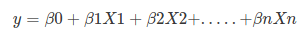
• Linear Regression Equation:

  • Where, y is dependent variable and x1, x2 ... and Xn are explanatory variables.

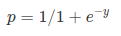
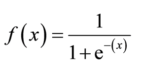
• Sigmoid Function:

  

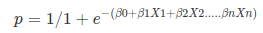
• Apply Sigmoid function on linear regression:

Properties of Logistic Regression:

• The dependent variable in logistic regression is between 0 and 1; Follows a sigmoid function
• Estimation is done through maximum likelihood.

10.3.1 Sigmoid Function

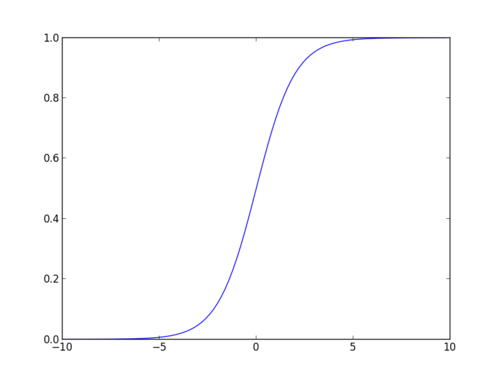
• The sigmoid function, also called logistic function gives an ‘S’ shaped curve that can take any real-valued number and map it into a value between 0 and 1.

• If the curve goes to positive infinity, y predicted will become 1, and if the curve goes to negative infinity, y predicted will become 0. If the output of the sigmoid function is more than 0.5, we can classify the outcome as 1 or YES, and if it is less than 0.5, we can classify it as 0 or NO.

• The outputcannot For example: If the output is 0.75, we can say in terms of probability as: There is a 75 percent chance that a propect will convert to a customers

11.5 Building a Logistic Regession Model

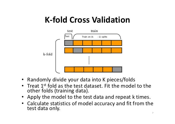
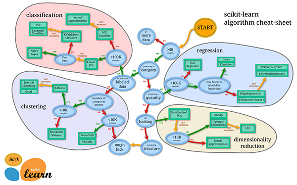
Several Steps needs to be followed for building a classification model

• Data Wrangling and cleaning from week 10
• Categorical variable treatment
  • Ordinal -> order integer mapping
  • Dummy Variable Creation
• Test Train Split
• Model Development using sci-kit learn

df.columns

Index(['prospsid', 'leadnum', 'origin', 'dne', 'dnc', 'target', 'totviz',
       'tos', 'pageviz', 'lastact', 'country', 'splz', 'leadsrc', 'curoccp',
       'reason', 'srch', 'mag', 'newsart', 'edforum', 'newsad', 'digitalad',
       'reco', 'updates', 'tag', 'leadquality', 'supchncont', 'dmcontent',
       'leadprofile', 'city', 'asymactidx', 'asymprofidx', 'asymactscr',
       'asymprofscr', 'chkpay', 'freecp', 'lastnotact'],
      dtype='object')

11.5.1 Variables to build model

• To keep things simple we shall use a small group of categorical and continuous variable
• I am going to clean them as shown in the previous class using a few functions
• These functions are generic enough to be repurposed for any logistic regression exercise that you may encounter

features = ['origin', 'splz', 'totviz','tos', 'pageviz']

10.4.1.1 Test for NULLs

NULL_Thres= 30
features= df.loc[:, features].isnull().sum()[df.loc[:, features].isnull().sum()/len(df)< NULL_Thres].index.tolist()

10.4.1.2 split into categorical and numerical variables

cat_vars= df.loc[:, features].dtypes[df.loc[:, features].dtypes=='object'].index.tolist()
num_vars= df.loc[:, features].dtypes[df.loc[:, features].dtypes!='object'].index.tolist()

cat_vars

['origin', 'splz']

num_vars

['totviz', 'tos', 'pageviz']

11.5.2 Categorical Variable cleaning

#cat_col= 'origin'
#thres= .1
def prep_cat(df, cat_col, thres=.1):
  '''
  Takes a pandas dataframe, categorical column name and threshold as a input and provides a dataframe as a output
  The output dataframe's cat column goes through he following transformation:
  1. Converted to all lower case
  2. NULLs replaced with Mode
  3. Categories in the variable that are < a threshold [default set to 10%] are all grouped as 'others'
  '''
  #1
  df[cat_col]= df.loc[:, cat_col].str.lower()
  #2
  df.loc[:, cat_col].fillna(df.loc[:, cat_col].mode()[0], inplace= True)
  #3
  smalls= df.loc[:, cat_col].value_counts(normalize=True)[df.loc[:, cat_col].value_counts(normalize=True) < thres].index.tolist()
  small_map= dict(zip(smalls, (len(smalls)*'others ').split(' ')[:-1]))
  df[cat_col]= df.loc[:, cat_col].map(small_map).fillna(df.loc[:, cat_col])
  return(df)

df.origin.value_counts(normalize=True)

Google               0.311604
Direct Traffic       0.276293
Olark Chat           0.190678
Organic Search       0.125380
Reference            0.058018
Welingak Website     0.015428
Referral Sites       0.013581
Facebook             0.005976
bing                 0.000652
google               0.000543
Click2call           0.000435
Press_Release        0.000217
Live Chat            0.000217
Social Media         0.000217
testone              0.000109
Pay per Click Ads    0.000109
welearnblog_Home     0.000109
blog                 0.000109
NC_EDM               0.000109
WeLearn              0.000109
youtubechannel       0.000109
Name: origin, dtype: float64

for c in cat_vars:
  df= prep_cat(df, c, .1)
  print(c)
  print()
  print(df.loc[:, c].value_counts())

origin

google            2909
direct traffic    2543
olark chat        1755
organic search    1154
others             879
Name: origin, dtype: int64
splz

others                4884
select                3380
finance management     976
Name: splz, dtype: int64

11.5.3 Numerical Variable cleaning

def prep_num(cf, num_col, flr_cel=['5%','95%']):
  '''
  Takes a pandas dataframe, numerical column name and floor/ceiling percentile threshold as a input and provides a dataframe as a output
  The output dataframe's cat column goes through he following transformation:
  1. NULLs replaced with median
  2. Treat outliers- floor at flr_cel[0] and cap at flr_cel[1] percentile values
  '''
  df.loc[:,num_col].fillna(df.loc[:,num_col].median(), axis=0, inplace= True)
  p5=df.loc[:,num_col].describe(percentiles=[.05,.25,.50,.75,.95]).loc[flr_cel[0]]
  p95= df.loc[:,num_col].describe(percentiles=[.05,.25,.50,.75,.95]).loc[flr_cel[1]]
  df[num_col] = np.where(df[num_col] <p5, p5,df[num_col])
  df[num_col] = np.where(df[num_col] >p95, p95,df[num_col])
  return(df)

print(df.loc[:, c].describe())
for c in num_vars:
  df= prep_num(df, c)
  print(c)
  print()
  print(df.loc[:, c].describe())

count       9240
unique         3
top       others
freq        4884
Name: splz, dtype: object
totviz

count    9240.000000
mean        3.179221
std         2.761219
min         0.000000
25%         1.000000
50%         3.000000
75%         5.000000
max        10.000000
Name: totviz, dtype: float64
tos

count    9240.000000
mean      479.244156
std       528.819773
min         0.000000
25%        12.000000
50%       248.000000
75%       936.000000
max      1562.000000
Name: tos, dtype: float64
pageviz

count    9240.000000
mean        2.255105
std         1.779471
min         0.000000
25%         1.000000
50%         2.000000
75%         3.000000
max         6.000000
Name: pageviz, dtype: float64

11.5.4 Categorical Vairable treatment

• Recall that the categorical variables are literal string
• For nominal variables- they are encoded as summy variables or 0/1
• Ordinal variables may be mapped to integers of increasing order. We had examples from week 9 visualization class

11.5.4.1 Dummy Variables

features.append('target')

mf= pd.get_dummies(df.loc[:, features], columns= cat_vars)

mf.columns

Index(['totviz', 'tos', 'pageviz', 'target', 'origin_direct traffic',
       'origin_google', 'origin_olark chat', 'origin_organic search',
       'origin_others', 'splz_finance management', 'splz_others',
       'splz_select'],
      dtype='object')

df.loc[:, features].head()

	origin	splz	totviz	tos	pageviz
Prospect ID
7927b2df-8bba-4d29-b9a2-b6e0beafe620	olark chat	select	0.0	0.0	0.0
2a272436-5132-4136-86fa-dcc88c88f482	organic search	select	5.0	674.0	2.5
8cc8c611-a219-4f35-ad23-fdfd2656bd8a	direct traffic	others	2.0	1532.0	2.0
0cc2df48-7cf4-4e39-9de9-19797f9b38cc	direct traffic	others	1.0	305.0	1.0
3256f628-e534-4826-9d63-4a8b88782852	google	select	2.0	1428.0	1.0

mf.head()

	totviz	tos	pageviz	target	origin_direct traffic	origin_google	origin_olark chat	origin_organic search	origin_others	splz_finance management	splz_others	splz_select
Prospect ID
7927b2df-8bba-4d29-b9a2-b6e0beafe620	0.0	0.0	0.0	0	0	0	1	0	0	0	0	1
2a272436-5132-4136-86fa-dcc88c88f482	5.0	674.0	2.5	0	0	0	0	1	0	0	0	1
8cc8c611-a219-4f35-ad23-fdfd2656bd8a	2.0	1532.0	2.0	1	1	0	0	0	0	0	1	0
0cc2df48-7cf4-4e39-9de9-19797f9b38cc	1.0	305.0	1.0	0	1	0	0	0	0	0	1	0
3256f628-e534-4826-9d63-4a8b88782852	2.0	1428.0	1.0	1	0	1	0	0	0	0	0	1

plt.figure(figsize=(10,10))
sns.heatmap(mf.corr(), annot=True)
plt.show()

mf.corr().target.abs().sort_values(ascending= False)

target                     1.000000
tos                        0.365876
origin_others              0.260910
splz_select                0.154025
origin_olark chat          0.129459
splz_others                0.121951
origin_direct traffic      0.080682
totviz                     0.045568
splz_finance management    0.043308
origin_google              0.026286
origin_organic search      0.005879
pageviz                    0.005289
Name: target, dtype: float64

final_features= mf.corr().target.abs().sort_values(ascending= False).index.tolist()

final_features

['target',
 'tos',
 'origin_others',
 'splz_select',
 'origin_olark chat',
 'splz_others',
 'origin_direct traffic',
 'totviz',
 'splz_finance management',
 'origin_google',
 'origin_organic search',
 'pageviz']

10.6 Training the Model

• We will use the standard python library sci-kit learn also called sklearn to build logistic regression model

• We shall instantiate differrent modules and submodule of the module to build the logistic regresion model and examine it's effectiveness

mf.isnull().sum()[mf.isnull().sum()> 0]

Series([], dtype: int64)

2 Feature Model

• Just to keep things simple
• You can add as many dependent variables you like

set1= ['tos','totviz']

X= mf[set1]
y= mf.target

10.6.1 Train Test Split

• train data set: Train the ML model on this portion of the data
• test data set: Blind data set to test efficiency of ML model thus developed

from sklearn.model_selection import train_test_split
X_train, X_test, y_train, y_test = train_test_split(X, y,test_size=0.25, random_state=42)

10.6.2 Fitting a Model

# import the class
from sklearn.linear_model import LogisticRegression

# instantiate the model (using the default parameters)
logreg = LogisticRegression()
# fit the model with data
logreg.fit(X_train,y_train)
#
y_hat=logreg.predict(X_test)

# Create Ranges of Values
x_min, x_max = X_test.iloc[:, 0].min() - .5, X_test.iloc[:, 0].max() + .5
y_min, y_max = X_test.iloc[:, 1].min() - .5, X_test.iloc[:, 1].max() + .5

# Create Meshgrid for above range and 
h = .02  # step size in the mesh
xx, yy = np.meshgrid(np.arange(x_min, x_max, h), np.arange(y_min, y_max, h))
Z = logreg.predict(np.c_[xx.ravel(), yy.ravel()])
Z = Z.reshape(xx.shape)
plt.figure(1, figsize=(10,7))
plt.pcolormesh(xx, yy, Z, cmap=plt.cm.Set1)

# Plot also the X_test points
plt.scatter(X_test.iloc[:, 0], X_test.iloc[:, 1], c=y_test, edgecolors='k', cmap=plt.cm.Set1_r)
plt.xlabel('Time on Site')
plt.ylabel('Total Page Visited')

plt.xlim(xx.min(), xx.max())
plt.ylim(yy.min(), yy.max())
plt.xticks()
plt.yticks()
plt.grid(color='blue')
plt.show()

Note:-

Color Scheme Reversed

• Correctly Classified:
  • Grey on Red
  • Red on Grey

• Incorrectly Classified:

  • Red on Red
  • Grey on Grey

  Watch Out:- Color scheme reversed

10.7 Model Evaluation

Classification Models are evaluated with the help of Quality Metrics and not through visual inspection

Multivariate Model

The 2 feature model was built mostly for visualization.

Now using the same formulation we shall build a model with 5 features with the highest correlation

# Top 5 features with highest correlation
set2= final_features[1:6]
# creating X and y
X= mf[set2]
y= mf.target
# Train Test split- using pre-loaded modules
X_train, X_test, y_train, y_test = train_test_split(X, y,test_size=0.25, random_state=42)
logreg = LogisticRegression()
# fit the model with data
logreg.fit(X_train,y_train)
#
y_hat=logreg.predict(X_test)

set2

['tos', 'origin_others', 'splz_select', 'origin_olark chat', 'splz_others']

10.7.1 Model Parameters

logreg.coef_

array([[ 1.95304724e-03,  2.89142383e+00, -8.01994497e-01,
         1.07904692e+00, -2.13862799e-02]])

logreg.intercept_

array([-1.65510334])

logreg.predict_proba(X_test)

array([[0.76186569, 0.23813431],
       [0.4655817 , 0.5344183 ],
       [0.92079454, 0.07920546],
       ...,
       [0.3142452 , 0.6857548 ],
       [0.37360491, 0.62639509],
       [0.81788118, 0.18211882]])

0.76186569+ 0.23813431

1.0

10.7.2 Confusion Matrix

A confusion matrix is a table that is used to evaluate the performance of a classification model. You can also visualize the performance of an algorithm. The fundamental of a confusion matrix is the number of correct and incorrect predictions are summed up class-wise

from sklearn import metrics
cnf_matrix = metrics.confusion_matrix(y_test, y_hat)
cnf_matrix

array([[1190,  214],
       [ 339,  567]])

class_names=[1,0] # name  of classes
fig, ax = plt.subplots()
tick_marks = np.arange(len(class_names))
plt.xticks(tick_marks, class_names)
plt.yticks(tick_marks, class_names)
# create heatmap
sns.heatmap(pd.DataFrame(cnf_matrix), annot=True, cmap="YlOrRd" ,fmt='g')
ax.xaxis.set_label_position("top")
plt.tight_layout()
plt.title('Confusion matrix', y=1.1)
plt.ylabel('Actual label')
plt.xlabel('Predicted label')

Text(0.5, 257.44, 'Predicted label')

10.7.3 Precision & Recall

print("Accuracy:",metrics.accuracy_score(y_test, y_hat))
print("Precision:",metrics.precision_score(y_test, y_hat))
print("Recall:",metrics.recall_score(y_test, y_hat))

Accuracy: 0.7606060606060606
Precision: 0.7259923175416133
Recall: 0.6258278145695364

10.7.3 Receiver Operating Characteristic(ROC)

Receiver Operating Characteristic(ROC) curve is a plot of the true positive rate against the false positive rate. It shows the tradeoff between sensitivity and specificity

y_pred_proba = logreg.predict_proba(X_test)[::,1]
fpr, tpr, _ = metrics.roc_curve(y_test,  y_pred_proba)
auc = metrics.roc_auc_score(y_test, y_pred_proba)
plt.figure(figsize=(7,7))
plt.plot(fpr,tpr,label="X_test, auc="+str(auc))
plt.legend(loc=4)
plt.grid(color='gray')
plt.xlabel('False Positive Rate')
plt.ylabel('True Positive Rate')
plt.show()

10.8 Important Concepts at a High Level

10.8.1 Overfitting versus Underfitting

10.8.2 Bias Variance Tradeoff

10.8.3 Cross-Validation

• K= n,5,10 are popular

10.8.4 Leakage

• Data leakage (or leakage) happens when your training data contains information about the target, but similar data will not be available when the model is used for prediction.

• This leads to high performance on the training set (and possibly even the validation data), but the model will perform poorly in production.

• To prevent this type of data leakage, any variable updated (or created) after the target value is realized should be excluded.